4.4 SR–GR matching

To determine the calibration bias of each radar, we employ the relative calibration approach by using the spaceborne-radar (SR) as a reference. In order to avoid introducing errors by interpolation, we use a volume-matching procedure. The 3D geometric matching method proposed by Schwaller and Morris (2011), further developed by Warren et al. (2018), was used to match SR bins to GR bins. This method has been implemented with the Subic radar for the same time period by Crisologo et al. (2018). In this study, we extend it to the TAG radar. Since the two radars are operating under the same scanning strategy and spatial resolution, the thresholds applied in filtering the data are kept the same as in the SR–SUB comparison described in Section 3.2 Table 3 of Crisologo et al. (2018). Details of the SR data specifications and the matching procedure can be found in Crisologo et al. (2018).

4.4.1 GR–GR matching

We compare the reflectivities of both ground radars in the overlapping region to quantify the mean and the standard deviation of their differences, and thus the effectiveness of the quality-weighting and the relative calibration procedure. In order to compare reflectivities from different radars, the different viewing geometries must be carefully considered. The polar coordinates of each radar are transformed into azimuthal equidistant projection coordinates, centered on each radar. Each radar cartesian coordinate is then transformed into the other radar’s spherical coordinate system, such that each of the radar bins of the TAG radar have coordinates with respect to the SUB radar, and vice versa. For this purpose, we use the georeferencing module of the wradlib library (https://wradlib.org) which allows for transforming between any spherical and Cartesian reference systems. Bins of the TAG radar that are less than 120 km away from the SUB radar are chosen. The same is done for bins of the SUB radar. In order to match only bins of similar volume, Seo, Krajewski, and Smith (2014) suggested a matching zone of 3 km within the equidistant line between the two radars. We decided to make this requirement less strict in order to include more matches, and thus extended this range to 10 km. From the selected bins, each SUB bin is matched with the closest TAG bin, not exceeding 250 m in distance. The matching SUB and TAG bins are exemplarily shown in black in Figure 4.3 for the 0.5\(^{\circ}\) elevation angle, such that each black bin in the SUB row corresponds with a black bin in the TAG row.

4.4.2 Estimation of path-integrated attenuation

Atmospheric attenuation depends on the radar’s operating frequency Holleman et al. (2006). For radar signals with wavelengths below 10 cm (such as C- and X-band radars), significant attenuation due to precipitation can occur Vulpiani et al. (2006), depending on precipitation intensity Holleman et al. (2006). In tropical areas such as the Philippines, where torrential rains and typhoons abound, C-band radars suffer from substantial PIA.

In this study, we require PIA estimates as a quality variable to assign different weights of GR reflectivity samples when computing quality-weighted averages of reflectivity (see section 4.4.4). For that purpose, PIA is estimated by using dual-pol moments observed by the TAG radar. The corresponding procedure includes the removal of non-meteorological echoes based on a fuzzy echo classification, and the reconstruction of the differential propagation phase from which PIA is finally estimated. The method is based on Vulpiani et al. (2012), and was comprehensively documented and verified for the TAG radar by Crisologo et al. (2014) which is why we only briefly outline it in the following.

The fuzzy classification of meteorological vs. non-meteorological echoes was based on the following decision variables: the Doppler velocity, the copolar cross-correlation, the textures (Gourley, Tabary, and Parent du Chatelet 2007) of differential reflectivity, copolar cross-correlation, and differential propagation phase (\(\Phi_{DP}\)), and a static clutter map. The parameters of the trapezoidal membership functions as well as the weights of the decision variables are specified in Table 2 of Crisologo et al. (2014). Bins classified as non-meteorological were removed from the beam profile and then filled in the subsequent processing step. In that step, a clean \(\Phi_{DP}\) profile is reconstructed by removing the effects of wrapping, system offset and residual artifacts. The reconstruction consists of an iterative procedure in which \(K_{DP}\) is repeatedly estimated from \(\Phi_{DP}\) using a convolutional filter, and \(\Phi_{DP}\) again retrieved from \(K_{DP}\) via integration, after filtering spurious and physically implausible \(K_{DP}\) values.

According to Bringi et al. (1990), specific attenuation, \(\alpha_{hh}\) (dB km\(^{-1}\)), is linearly related to \(K_{DP}\) by a coefficient \(\gamma_{hh}\) (dB deg\(^{-1}\)) which we assume to be constant in time and space with a value of \(\gamma_{hh}\) = 0.08 (Carey et al. 2000). Hence, the two-way path-integrated attenuation, \(A_{hh}\) (dB), can then be obtained from the integral of the specific attenuation along each beam—which is equivalent to our reconstructed \(\Phi_{DP}\) from which the system offset (\(\Phi_{DP}(r_0)\)) was removed in the previous step.

\[ \begin{align} A_{hh}(s) &= 2 \int ^r _{r_0} \alpha_{hh}(s)ds \\ &= 2 \gamma_{hh} \int^r_{r_0} K_{DP}(s)ds \\ &= \gamma_{hh} (\Phi_{DP}(r) - \Phi_{DP} (r_0)) \end{align} \]

4.4.3 Beam Blockage

In regions of complex topography, the ground radar beam can be totally or partially blocked by topographic obstacles, resulting in weakening or loss of the signal. To simulate the extent of beam blockage for each ground radar, as introduced by topography, we used the algorithm proposed by Bech et al. (2003), together with the Shuttle Radar Topography Mission (SRTM) DEM with a 1 arc-second (approximately 30 m) resolution. The procedure has been documented in Crisologo et al. (2018) in more detail. In summary, the values of the DEM are resampled to the radar bin centroid coordinates to match the polar resolution of the radar data. Then, the algorithm computes the beam blockage fraction for each radar bin by comparing the elevation of the radar beam in that bin with the terrain elevation. Finally, the cumulative beam blockage fraction (BBF) is calculated for all the bins along each ray, where a value of 1.0 corresponds to total occlusion and a value of 0.0 to complete visibility.

4.4.4 Quality index and quality-weighted averaging

The quality index is a quantity used to describe data quality, represented by numbers ranging from 0 (poor quality) to 1 (excellent quality), with the objective of characterizing data quality independent of the source, hardware, and signal processing (Einfalt, Szturc, and Ośródka 2010).

To calculate a quality index for the beam blockage fraction, the transformation function suggested by Zhang et al. (2011) is used:

\[ \begin{equation} \scriptstyle Q_{BBF} = \left\{ \begin{matrix} 1 & BBF \leq 0.1 \\ 1-\frac{BBF-0.1}{0.4} & 0.1 < BBF \leq 0.5\\ 0 & BBF > 0.5 \end{matrix} \right\} \end{equation} \]

Figure @ref(fig:Fig3_matched_BBF_05) shows the beam blockage quality index (\(Q_{BBF}\)) maps of SUB and TAG for the lowest elevation angle. Subic is substantially affected by beam blockage in the northern and southern sector, due to the radar sitting between two mountains along a mountain range. The southern beam blockage sector of the Subic radar clearly affects the region of overlap with the Tagaytay radar. Meanwhile, TAG has a clearer view towards the north, with only a narrow sector to the east and partially in the south being affected by very high beam blockage. It is not shown in the figure, but the higher elevation angles of the TAG radar are not affected by any beam blockage.

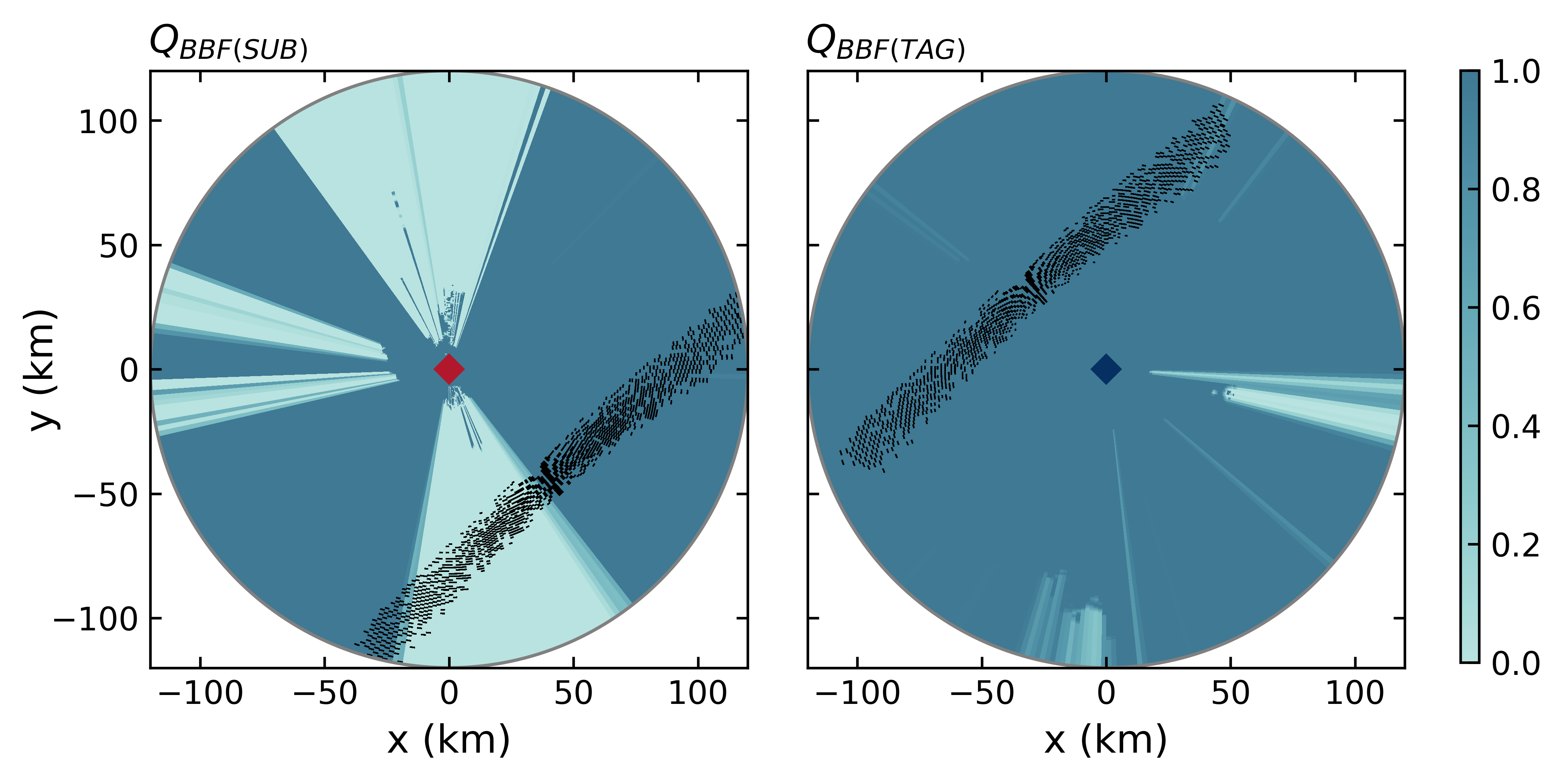
Figure 4.3: The beam blockage quality index (\(Q_{BBF}\)) for the two radars is shown in the background for each corresponding elevation angle. Black points show the locations of matched bins between SUB and TAG for each radar coverage, exemplarily for an elevation of 0.5 degree

For path-integrated attenuation, the values are transformed into a quality index as

\[ \begin{equation} \scriptstyle Q_{PIA} = \left\{\begin{matrix} 1 & \text{for} & K_{r,s} < K_{min}\\ 0 & \text{for} & K_{r,s} > K_{max}\\ \frac{K_{max} - K_{r,s}}{K_{max} - K_{min}} & \text{else}, & \end{matrix}\right\} \end{equation} \]

following the function proposed by Friedrich, Hagen, and Einfalt (2006), where \(K_{min}\) and \(K_{max}\) are the lower and upper attenuation thresholds. The values for \(K_{min}\) and \(K_{max}\) are chosen to be 1 dB and 10 dB.

Multiple quality indices from different quality variables can be combined in order to obtain a single index of total quality. Different combination approaches have been suggested, e.g. by addition or multiplication (Norman et al. 2010), or by weighted averaging (Michelson et al. 2005). We chose to combine \(Q_{BBF}\) and \(Q_{PIA}\) multiplicatively, in order to make sure that a low value of either of the two propagates to the total quality index (\(Q_{GR} = Q_{GR,BBF} * Q_{GR,PIA}\)), where \(Q_{GR}\) can either be \(Q_{SUB}\) or \(Q_{TAG}\).

It should be noted that \(Q_{SUB,PIA}\) is always considered to have a value of 1, as we consider attenuation negligible for S-band radars, so that effectively \(Q_{SUB}\) = \(Q_{SUB,BBF}\).

Based on this quality index \(Q_{GR}\), we follow the quality-weighting approach as outlined in Crisologo et al. (2018). For each match between SR and GR bins, the quality \(Q_{match}\) is obtained from the minimum \(Q_{GR}\) value of the GR bins in that match. We then compute the average and the standard deviation of the reflectivity differences between SR and GR by using the Qmatch values as linear weights (see Crisologo et al. (2018) for details). We basically follow the same approach when we compute the quality-weighted average and standard deviation of the differences between the two ground radars, SUB and TAG, in the region of overlap. Here, the quality \(Q_{match}\) of each match is computed as the product \(Q_{SUB}*Q_{TAG}\) of the two matched GR bins.

It should be emphasized at this point that, in the region of overlap, the TAG radar is not affected by beam blockage. So while the computation of calibration bias for the TAG radar, based on SR overpasses, is affected by \(Q_{TAG,BBF}\) (as it uses the full TAG domain), the comparison of SUB and TAG reflectivities is, in fact, only governed by \(Q_{SUB,BBF}\) and \(Q_{TAG,PIA}\).

4.4.5 Computational details

Following the guidelines for transparency and reproducibility in weather and climate sciences as suggested by Irving (2016), we have made the entire processing workflow and sample data available online at https://github.com/IreneCrisologo/inter-radar. The main components of that workflow are based on the open source software library for processing weather radar data called wradlib (M. Heistermann, Jacobi, and Pfaff 2013), version 1.2 (released on 31.10.2018) based on Python 3.6. The main dependencies of wradlib include Numerical Python (NumPy; Oliphant (2015), Matplotlib (Hunter 2007), Scientific Python (SciPy; Jones, Oliphant, and Peterson (2014)), h5py (Collette 2013), netCDF4 (Rew et al. 1989), gdal (GDAL Development Team 2017), and pandas (McKinney 2010).

References

Bech, Joan, Bernat Codina, Jeroni Lorente, and David Bebbington. 2003. “The Sensitivity of Single Polarization Weather Radar Beam Blockage Correction to Variability in the Vertical Refractivity Gradient.” Journal of Atmospheric and Oceanic Technology 20 (6): 845–55. http://journals.ametsoc.org/doi/abs/10.1175/1520-0426(2003)020%3C0845:TSOSPW%3E2.0.CO;2.

Bringi, V. N., V. Chandrasekar, N. Balakrishnan, and D. S. Zrnić. 1990. “An Examination of Propagation Effects in Rainfall on Radar Measurements at Microwave Frequencies.” Journal of Atmospheric and Oceanic Technology 7 (6): 829–40. https://doi.org/10.1175/1520-0426(1990)007<0829:AEOPEI>2.0.CO;2.

Carey, Lawrence D., Steven A. Rutledge, David A. Ahijevych, and Tom D. Keenan. 2000. “Correcting Propagation Effects in C-Band Polarimetric Radar Observations of Tropical Convection Using Differential Propagation Phase.” Journal of Applied Meteorology 39 (9): 1405–33. https://doi.org/10.1175/1520-0450(2000)039<1405:CPEICB>2.0.CO;2.

Collette, Andrew. 2013. Python and HDF5. O’Reilly.

Crisologo, Irene, Robert A. Warren, Kai Mühlbauer, and Maik Heistermann. 2018. “Enhancing the Consistency of Spaceborne and Ground-Based Radar Comparisons by Using Beam Blockage Fraction as a Quality Filter.” Atmospheric Measurement Techniques 11 (9): 5223–36. https://doi.org/https://doi.org/10.5194/amt-11-5223-2018.

Crisologo, I., G. Vulpiani, C. C. Abon, C. P. C. David, A. Bronstert, and Maik Heistermann. 2014. “Polarimetric Rainfall Retrieval from a C-Band Weather Radar in a Tropical Environment (the Philippines).” Asia-Pacific Journal of Atmospheric Sciences 50 (S1): 595–607. https://doi.org/10.1007/s13143-014-0049-y.

Einfalt, Thomas, Jan Szturc, and Katarzyna Ośródka. 2010. “The Quality Index for Radar Precipitation Data: A Tower of Babel?” Atmospheric Science Letters 11 (2): 139–44. https://doi.org/10.1002/asl.271.

Friedrich, Katja, Martin Hagen, and Thomas Einfalt. 2006. “A Quality Control Concept for Radar Reflectivity, Polarimetric Parameters, and Doppler Velocity.” Journal of Atmospheric and Oceanic Technology 23 (7): 865–87. http://journals.ametsoc.org/doi/abs/10.1175/JTECH1920.1.

GDAL Development Team. 2017. “GDAL - Geospatial Data Abstraction Library, Version 2.2.3.” Open Source Geospatial Foundation. http://www.gdal.org/.

Gourley, Jonathan J., Pierre Tabary, and Jacques Parent du Chatelet. 2007. “A Fuzzy Logic Algorithm for the Separation of Precipitating from Nonprecipitating Echoes Using Polarimetric Radar Observations.” Journal of Atmospheric and Oceanic Technology 24 (8): 1439–51. https://doi.org/10.1175/JTECH2035.1.

Heistermann, M., S. Jacobi, and T. Pfaff. 2013. “Technical Note: An Open Source Library for Processing Weather Radar Data (Wradlib).” Hydrology and Earth System Sciences 17 (2): 863–71. https://doi.org/10.5194/hess-17-863-2013.

Holleman, Iwan, Daniel Michelson, Gianmario Galli, Urs Germann, and Markus Peura. 2006. “Quality Information for Radars and Radar Data.” OPERA workpackage 1.2. http://cdn.knmi.nl/system/data_center_publications/files/000/046/931/original/opera_wp12_v6.pdf?1432896393.

Hunter, J. D. 2007. “Matplotlib: A 2D Graphics Environment.” Computing in Science Engineering 9 (3): 90–95. https://doi.org/10.1109/MCSE.2007.55.

Irving, Damien. 2016. “A Minimum Standard for Publishing Computational Results in the Weather and Climate Sciences.” Bulletin of the American Meteorological Society 97 (7): 1149–58. https://doi.org/10.1175/BAMS-D-15-00010.1.

Jones, Eric, Travis E. Oliphant, and Pearu Peterson. 2014. “SciPy: Open Source Scientific Tools for Python.”

McKinney, Wes. 2010. “Data Structures for Statistical Computing in Python.” In Proceedings of the 9th Python in Science Conference, 445:51–56. Austin, TX.

Michelson, Daniel, Thomas Einfalt, Iwan Holleman, Uta Gjertsen, Friedrich, Katja, Günther Haase, Magnus Lindskog, and Anna Jurczyk. 2005. Weather Radar Data Quality in Europe Quality Control and Characterisation. Luxembourg: Publications Office.

Norman, K., N. Gaussiat, D. Harrison, R. Scovell, and M. Boscacci. 2010. “A Quality Index for Radar Data.” OPERA Deliverable OPERA_2010_03. http://www.eumetnet.eu/sites/default/files/OPERA_2010_03_Quality_Index.pdf.

Oliphant, Travis E. 2015. Guide to NumPy. 2nd ed. USA: CreateSpace Independent Publishing Platform.

Rew, Russ, Glenn Davis, Steve Emmerson, Cathy Cormack, John Caron, Robert Pincus, Ed Hartnett, Dennis Heimbigner, Lynton Appel, and Ward Fisher. 1989. “Unidata NetCDF.” UCAR/NCAR - Unidata. http://www.unidata.ucar.edu/software/netcdf/.

Schwaller, Mathew R., and K. Robert Morris. 2011. “A Ground Validation Network for the Global Precipitation Measurement Mission.” Journal of Atmospheric and Oceanic Technology 28 (3): 301–19. https://doi.org/10.1175/2010JTECHA1403.1.

Seo, Bong-Chul, Witold F. Krajewski, and James A. Smith. 2014. “Four-Dimensional Reflectivity Data Comparison Between Two Ground-Based Radars: Methodology and Statistical Analysis.” Hydrological Sciences Journal 59 (7): 1320–34. https://doi.org/10.1080/02626667.2013.839872.

Vulpiani, Gianfranco, Mario Montopoli, Luca Delli Passeri, Antonio G. Gioia, Pietro Giordano, and Frank S. Marzano. 2012. “On the Use of Dual-Polarized C-Band Radar for Operational Rainfall Retrieval in Mountainous Areas.” Journal of Applied Meteorology and Climatology 51 (2): 405–25. https://doi.org/10.1175/JAMC-D-10-05024.1.

Vulpiani, G., F. S. Marzano, V. Chandrasekar, A. Berne, and R. Uijlenhoet. 2006. “Rainfall Rate Retrieval in Presence of Path Attenuation Using C-Band Polarimetric Weather Radars.” Natural Hazards and Earth System Science 6 (3): 439–50. https://doi.org/10.5194/nhess-6-439-2006.

Warren, Robert A., Alain Protat, Steven T. Siems, Hamish A. Ramsay, Valentin Louf, Michael J. Manton, and Thomas A. Kane. 2018. “Calibrating Ground-Based Radars Against TRMM and GPM.” Journal of Atmospheric and Oceanic Technology, February. https://doi.org/10.1175/JTECH-D-17-0128.1.

Zhang, JIAN, YOUCUN Qi, K. Howard, C. Langston, and B. Kaney. 2011. “Radar Quality Index (RQI)—A Combined Measure of Beam Blockage and VPR Effects in a National Network.” In Proceedings, International Symposium on Weather Radar and Hydrology. http://www.nssl.noaa.gov/projects/q2/tutorial/images/mosaic/WRaH_Proceedings_Zhang-et-al_v3.pdf.