3.3 Method
3.3.1 Partial beam shielding and quality index based on beam blockage fraction
In an ideal situation, SR and GR should have the same measurements for the same volume of the atmosphere, as they are measuring the same target. However, observational differences may arise due to different view geometries, different operating frequencies, different environmental conditions of each instrument, and different processes along the propagation path of the beam. As pointed out before, we focus on beam blockage as an index of GR data quality.
In regions of complex topography, ground radars are typically affected by the effects of beam blockage, induced by the interaction of the beam with the terrain surface resulting in a weakening or even loss of the signal. To quantify that process within the Subic radar coverage, a beam blockage map is generated following the algorithm proposed by Bech et al. (2003). It assesses the extent of occultation using a digital elevation model (DEM). While Bech et al. (2003) used the GTOPO30 DEM at a resolution of around 1 km, higher DEM resolutions are expected to increase the accuracy of estimates of beam blockage fraction, as shown by Kucera, Krajewski, and Young (2004), in particular the near range of the radar (Cremonini, Moisseev, and Chandrasekar 2016). The DEM used in this study is from the Shuttle Radar Topography Mission (SRTM) data, with 1 arc-second (approximately 30-meter) resolution. The DEM was resampled to the coordinates of the radar bin centroids, using spline interpolation, in order to match the polar resolution of the radar data (500 m in range and 1\(^{\circ}\) in azimuth, extending to a maximum range of 120 km from the radar site; see Figure 3.1). A beam blockage map is generated for all available elevation angles.
The beam blockage fraction was calculated for each bin and each antenna pointing angle. The cumulative beam blockage was then calculated along each ray. A cumulative beam blockage fraction (BBF) of 1.0 corresponds to full occlusion, and a value of 0.0 to perfect visibility.
The quality index based on beam blockage fraction is then computed following Zhang et al. (2011) as
\[ \begin{equation} \scriptstyle Q_{BBF} = \begin{cases} 1 & BBF \leq 0.1\\ 1 - \frac{BBF - 0.1}{0.4} & 0.1 < BBF \leq 0.5\\ 0 & BBF > 0.5 \end{cases} \end{equation} \]
A slightly different formulation to transform partial beam blockage to a quality index has been presented in other studies (Figueras i Ventura and Tabary 2013; Fornasiero et al. 2005; Ośródka, Szturc, and Jurczyk 2014; Rinollo et al. 2013) where the quality is zero (0) if BBF is above a certain threshold, and then linearly increases to one (1) above that threshold. It should be noted that these approaches are equally valid and can be used in determining the quality index based on beam blockage.
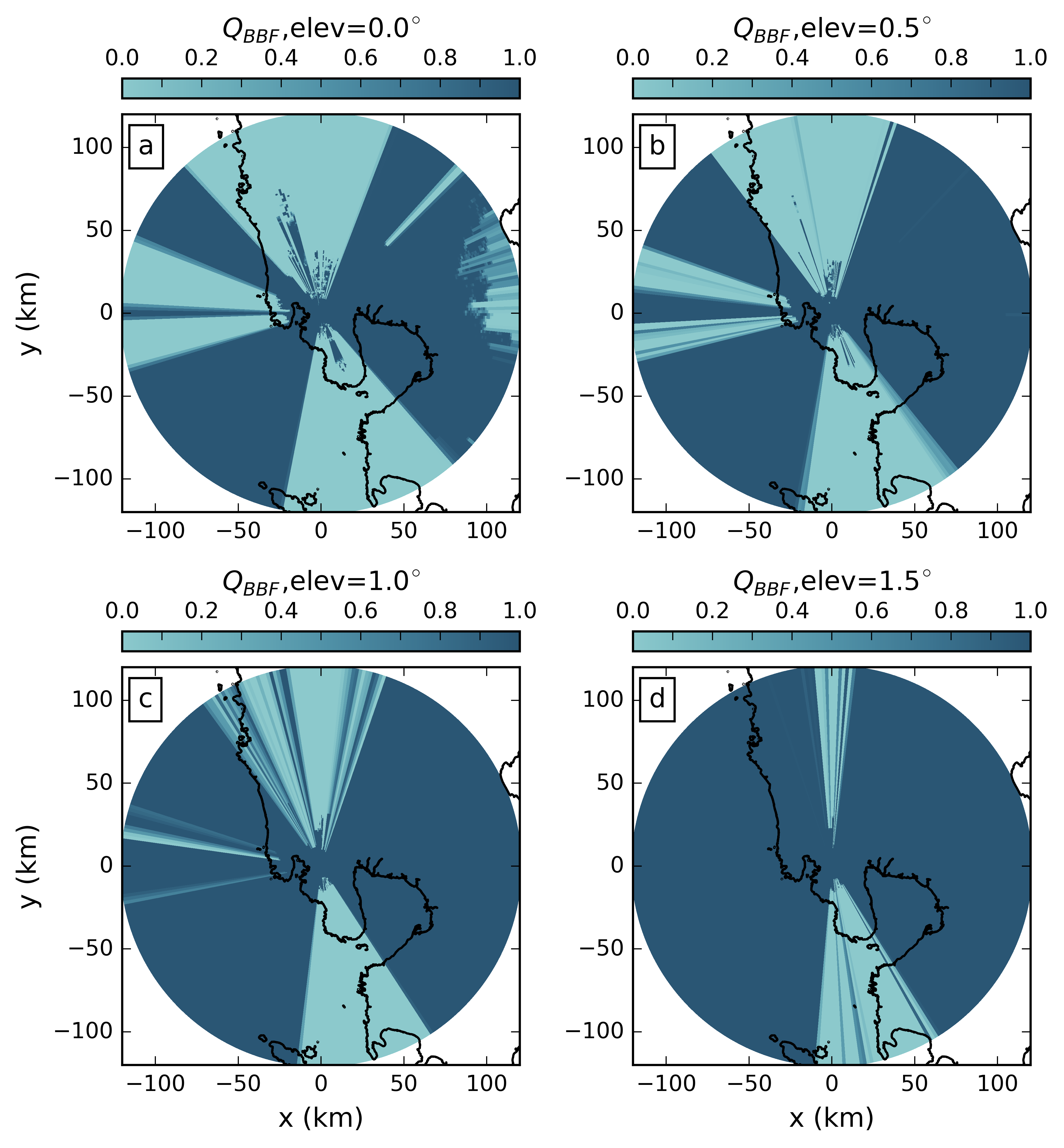
Figure 3.2: Quality index map of the beam blockage fraction for the Subic radar at (a) 0.0\(^{\circ}\), (b) 0.5\(^{\circ}\), (c) 1.0\(^{\circ}\), and (d) 1.5\(^{\circ}\) elevation angles.
Figure 3.2 shows the beam blockage map for the two lowest elevation angles of each scanning strategy. Figure 3.2a and c are for 0.0\(^{\circ}\) and 1.0\(^{\circ}\), which are the two lowest elevation angles in 2015, while Figure 3.2b and d are for 0.5\(^{\circ}\) and 1.5\(^{\circ}\), which are the two lowest elevation angles for the rest of the dataset.
As expected, the degree of beam blockage decreases with increasing antenna elevation, yielding the most pronounced beam blockage at 0.0\(^{\circ}\). Each blocked sector can be explained by the topography (see Figure 3.1), with the Zambales Mountains causing blockage in the northern sector, Mt. Natib in the southern sector, and the Redondo peninsula mountains in the western sector. The Sierra Madre also causes some partial beam blocking in the far east, and a narrow partial blocking northeast of the station where Mt. Arayat is located. As the elevation angle increases, the beam blockage becomes less pronounced or even disappears. Substantial blockage persists, however, for the higher elevation angles in the northern and southern sectors.
3.3.2 SR–GR Volume Matching
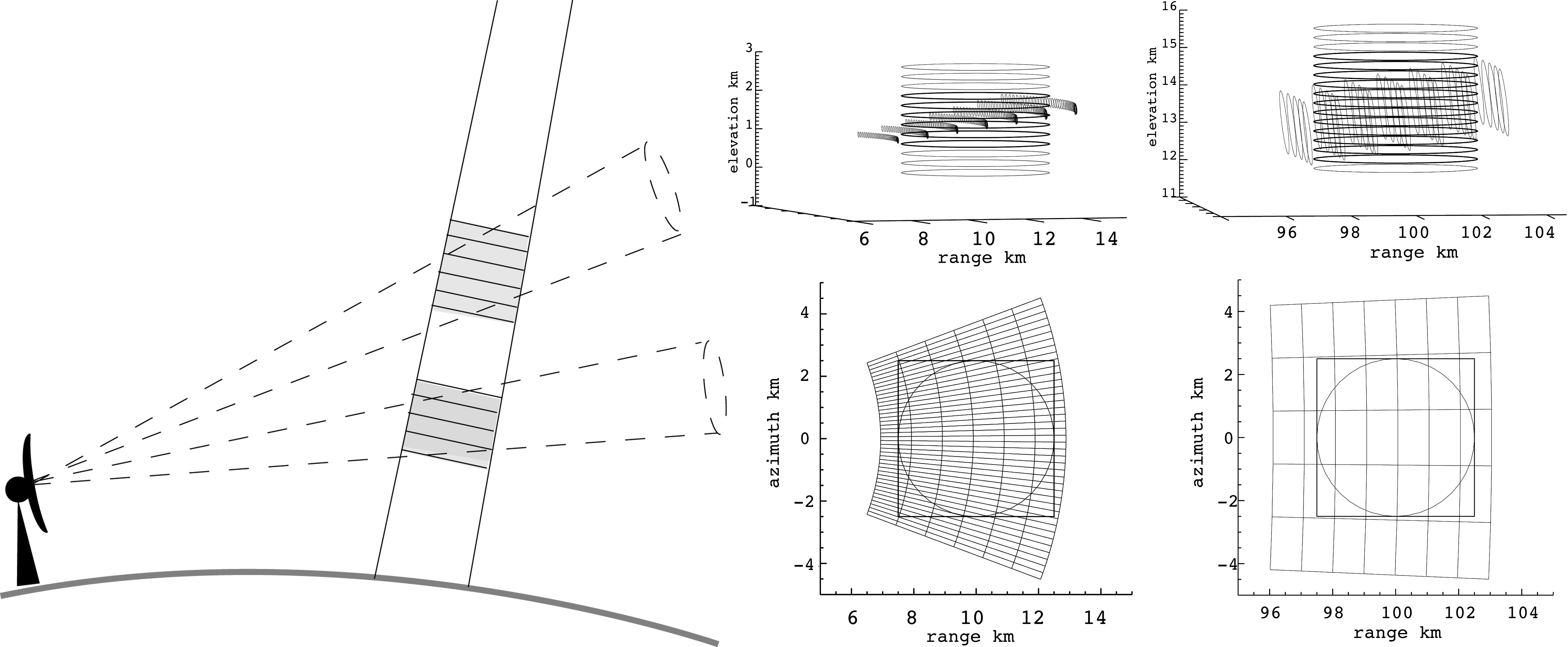
Figure 3.3: Diagram illustrating the geometric intersection. Left panel shows a single SR beam intersecting GR sweeps of two different elevation angles. The two top right panels illustrate the intersection of SR–GR sample volumes in the near and far ranges and the two bottom right panels show the projection of these intersections along an SR ray. From Schwaller and Morris (2011) (C) American Meteorological Society. Used with permission.
SR and GR data were matched only for the wet period within each year, which is from June to December. Several meta-data parameters were extracted from the TRMM 2A23 and GPM 2AKu products for each SR gate, such as the corresponding ray’s brightband height and width, gate coordinates in three dimensions (longitude and latitude of each ray’s Earth intercept and range gate index), time of overpass, precipitation type (stratiform, convective, or other), and rain indicators (rain certain or no-rain). The parallax-corrected altitude (above mean sea level) and horizontal location (with respect to the GR) of each gate were determined as outlined in the appendix of Warren et al. (2018). From the brightband height/width and the altitude of each SR gate, the brightband membership of each gate was calculated by grouping all rays in an overpass and computing the mean brightband height and width. A ratio value of less than zero indicates that the gate is below the brightband, and greater than one indicates that the gate is above the brightband, and a value between zero and one means that the gate is within the brightband. Only gates below and above the brightband were considered in the comparison. Warren et al. (2018) found a positive bias in GR–SR reflectivity difference for volume-matched samples within the melting layer, compared to those above and below the melting layer. They speculated that this was due to underestimation of the Ku- to S-band frequency correction for melting snow. In addition, while usually the samples above the brightband are used in GPM validation, there are significantly more samples below the melting layer, especially in a tropical environment such as the Philippines. To ensure that there are sufficient bins with actual rain included in the comparison, overpasses with less than 100 gates flagged as rain certain were discarded.
For each SR overpass, the GR sweep with the scan time closest to the overpass time within a 10-min window ($$5-min from overpass time) was selected. Both the SR and GR data were then geo-referenced into a common azimuthal equidistant projection centered on the location of the ground radar.
In order to minimize systematic differences in comparing the SR and GR reflectivities caused by the different measuring frequencies, the SR reflectivities were converted from Ku- to S-band following the formula:
\[ \begin{equation} Z(S) = Z(Ku) + \sum_{i=0}^4a_i [Z(Ku)]^i \end{equation} \]
where the \(a_i\) are the coefficients for dry snow and dry hail, rain, and in between at varying melting stages (Table 1 of Cao et al. (2013)). We used the coefficients for snow in the reflectivity conversion above the brightband, following Warren et al. (2018).
The actual volume matching algorithm closely follows the work of Schwaller and Morris (2011), where SR reflectivity is spatially and temporally matched with GR reflectivity without interpolation. The general concept is highlighted by Figure 3.3: each matching sample consists of bins from only one SR ray and one GR sweep. From the SR ray, those bins were selected that intersect with the vertical extent of a specific GR sweep at the SR ray location. From each GR sweep, those bins were selected that intersect with the horizontal footprint of the SR ray at the corresponding altitude. The SR and GR reflectivity of each matched volume was computed as the average reflectivity of the intersecting SR and GR bins.%, where the averaging is done in linear units (\(mm^6/m^3\)). %The entire workflow of this volume matching procedure is based on wradlib functions and available at https://github.com/wradlib/radargpm-beamblockage.
The nominal minimum sensitivity of both TRMM PR and GPM KuPR is 18 dBZ, so only values above this level were considered in the calculation of average SR reflectivity in the matched volume. In addition, the fraction of SR gates within a matched volume above that threshold was also recorded. On the other hand, all GR bins are included in the calculation of average GR reflectivity, after setting the bins with reflectivities below 0.0 dBZ to 0.0 dBZ, as suggested by Morris and Schwaller (2011). The filtering criteria applied in the workflow are summarized in Table 3.2.
| Criteria | Condition |
|---|---|
| Minimum number of pixels in overpass tagged as ’rain’ | 100 |
| Brightband membership | below or above |
| GR range limits (min–max) | 15 – 115 km |
| Minimum fraction of bins above minimum SR sensitivity | 0.7 |
| Minimum fraction of bins above minimum GR sensitivity | 0.7 |
| Maximum time difference between SR and GR | 5 min |
| Minimum PR reflectivity | 18 dBZ |
3.3.3 Assessment of the average reflectivity bias
Beam blockage and the corresponding GR quality maps were computed for each GR bin (cf. Section 3.3.1. For each matched SR–GR volume, the data quality was then based on the minimum quality of the GR bins in that volume.
To analyze the effect of data quality on the estimation of GR calibration bias, we compared two estimation approaches: a simple mean bias that does not take into account beam blockage, and a weighted mean bias that considers the quality value of each sample as weights. The corresponding standard deviation and weighted standard deviation were calculated as well. The overall process is summarized in Figure 3.4. In this way, we provide an overview of the variability of our bias estimates over time.
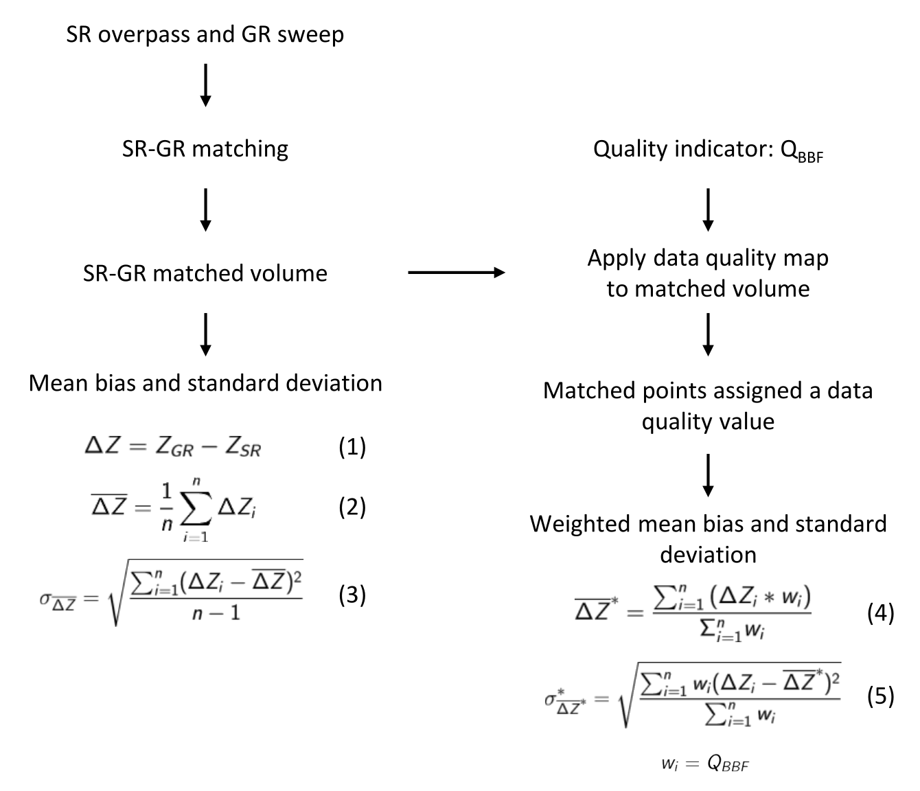
Figure 3.4: Flowchart describing the processing steps to calculate the mean bias and the weighted mean bias between ground radar data and satellite radar data.
3.3.4 Computational details
In order to promote transparency and reproducibility of this study, we mostly followed the guidelines provided by Irving (2016) which have also been implemented by a number of recent studies (Blumberg et al. 2017; Irving and Simmonds 2016; Rasp, Selz, and Craig 2018).
The entire processing workflow is based on wradlib (M. Heistermann, Jacobi, and Pfaff 2013), an extensively documented open-source software library for processing weather radar data. At the time of writing, we used version 1.0.0 released on 01 April 2018, based on Python 3.6. The main dependencies include Numerical Python (NumPy; Oliphant (2015)), Matplotlib (Hunter 2007), Scientific Python (SciPy; Jones, Oliphant, and Peterson (2014)), h5py (Collette 2013), netCDF4 (Rew et al. 1989), and gdal (GDAL Development Team 2017).
Reading the TRMM 2A23 and 2A25 version 7 data, GPM 2AKu version 5A data, and Subic ground radar data in the netCDF format converted through the EDGE software of EEC radars was done through the input-output module of wradlib. The beam blockage modelling is based on the Bech et al. (2003) method implemented as a function in wradlib’s data quality module. The volume-matching procedure is built upon the georeferencing and zonal statistics modules, accompanied by Pandas (McKinney 2010) for organizing and analysing the resulting database of matched bins. Visualization was carried out with the help of matplotlib (Hunter 2007) and Py-ART (Helmus and Collis 2016).
An accompanying GitHub repository that hosts the Jupyter notebooks of the workflow and sample data is made available at https://github.com/wradlib/radargpm-beamblockage.
References
Bech, Joan, Bernat Codina, Jeroni Lorente, and David Bebbington. 2003. “The Sensitivity of Single Polarization Weather Radar Beam Blockage Correction to Variability in the Vertical Refractivity Gradient.” Journal of Atmospheric and Oceanic Technology 20 (6): 845–55. http://journals.ametsoc.org/doi/abs/10.1175/1520-0426(2003)020%3C0845:TSOSPW%3E2.0.CO;2.
Blumberg, William G., Kelton T. Halbert, Timothy A. Supinie, Patrick T. Marsh, Richard L. Thompson, and John A. Hart. 2017. “SHARPpy: An Open-Source Sounding Analysis Toolkit for the Atmospheric Sciences.” Bulletin of the American Meteorological Society 98 (8): 1625–36. https://doi.org/10.1175/BAMS-D-15-00309.1.
Cao, Qing, Yang Hong, Youcun Qi, Yixin Wen, Jian Zhang, Jonathan J. Gourley, and Liang Liao. 2013. “Empirical Conversion of the Vertical Profile of Reflectivity from Ku-Band to S-Band Frequency.” Journal of Geophysical Research: Atmospheres 118 (4): 1814–25. https://doi.org/10.1002/jgrd.50138.
Collette, Andrew. 2013. Python and HDF5. O’Reilly.
Cremonini, Roberto, Dmitri Moisseev, and Venkatachalam Chandrasekar. 2016. “Airborne Laser Scan Data: A Valuable Tool with Which to Infer Weather Radar Partial Beam Blockage in Urban Environments.” Atmospheric Measurement Techniques 9 (10): 5063–75. https://doi.org/10.5194/amt-9-5063-2016.
Figueras i Ventura, Jordi, and Pierre Tabary. 2013. “The New French Operational Polarimetric Radar Rainfall Rate Product.” Journal of Applied Meteorology and Climatology 52 (8): 1817–35. https://doi.org/10.1175/JAMC-D-12-0179.1.
Fornasiero, A., P. P. Alberoni, R. Amorati, L. Ferraris, and A. C. Taramasso. 2005. “Effects of Propagation Conditions on Radar Beam-Ground Interaction: Impact on Data Quality.” Advances in Geosciences 2 (June): 201–8. https://hal.archives-ouvertes.fr/hal-00297387.
GDAL Development Team. 2017. “GDAL - Geospatial Data Abstraction Library, Version 2.2.3.” Open Source Geospatial Foundation. http://www.gdal.org/.
Heistermann, M., S. Jacobi, and T. Pfaff. 2013. “Technical Note: An Open Source Library for Processing Weather Radar Data (Wradlib).” Hydrology and Earth System Sciences 17 (2): 863–71. https://doi.org/10.5194/hess-17-863-2013.
Helmus, Jonathan, and Scott Collis. 2016. “The Python ARM Radar Toolkit (Py-ART), a Library for Working with Weather Radar Data in the Python Programming Language.” Journal of Open Research Software 4 (1). https://doi.org/10.5334/jors.119.
Hunter, J. D. 2007. “Matplotlib: A 2D Graphics Environment.” Computing in Science Engineering 9 (3): 90–95. https://doi.org/10.1109/MCSE.2007.55.
Irving, Damien. 2016. “A Minimum Standard for Publishing Computational Results in the Weather and Climate Sciences.” Bulletin of the American Meteorological Society 97 (7): 1149–58. https://doi.org/10.1175/BAMS-D-15-00010.1.
Irving, Damien, and Ian Simmonds. 2016. “A New Method for Identifying the Pacific–South American Pattern and Its Influence on Regional Climate Variability.” Journal of Climate 29 (17): 6109–25. https://doi.org/10.1175/JCLI-D-15-0843.1.
Jones, Eric, Travis E. Oliphant, and Pearu Peterson. 2014. “SciPy: Open Source Scientific Tools for Python.”
Kucera, Paul A., Witold F. Krajewski, and C. Bryan Young. 2004. “Radar Beam Occultation Studies Using GIS and DEM Technology: An Example Study of Guam.” Journal of Atmospheric and Oceanic Technology 21 (7): 995–1006. http://journals.ametsoc.org/doi/full/10.1175/1520-0426(2004)021%3C0995:RBOSUG%3E2.0.CO%3B2.
McKinney, Wes. 2010. “Data Structures for Statistical Computing in Python.” In Proceedings of the 9th Python in Science Conference, 445:51–56. Austin, TX.
Morris, Kenneth R., and Mathew Schwaller. 2011. “Sensitivity of Spaceborne and Ground Radar Comparison Results to Data Analysis Methods and Constraints.” In 35th Conference on Radar Meteorology. Pittsburgh, PA: American Meteorological Society. https://ams.confex.com/ams/35Radar/webprogram/Manuscript/Paper191729/AMS_35th_Radar_paper_final.pdf.
Oliphant, Travis E. 2015. Guide to NumPy. 2nd ed. USA: CreateSpace Independent Publishing Platform.
Ośródka, Katarzyna, Jan Szturc, and Anna Jurczyk. 2014. “Chain of Data Quality Algorithms for 3-D Single-Polarization Radar Reflectivity (RADVOL-QC System).” Meteorological Applications 21 (2): 256–70. https://doi.org/10.1002/met.1323.
Rasp, Stephan, Tobias Selz, and George C. Craig. 2018. “Variability and Clustering of Midlatitude Summertime Convection: Testing the Craig and Cohen Theory in a Convection-Permitting Ensemble with Stochastic Boundary Layer Perturbations.” Journal of the Atmospheric Sciences 75 (2): 691–706.
Rew, Russ, Glenn Davis, Steve Emmerson, Cathy Cormack, John Caron, Robert Pincus, Ed Hartnett, Dennis Heimbigner, Lynton Appel, and Ward Fisher. 1989. “Unidata NetCDF.” UCAR/NCAR - Unidata. http://www.unidata.ucar.edu/software/netcdf/.
Rinollo, A., G. Vulpiani, S. Puca, P. Pagliara, J. Kaňák, E. Lábó, L’. Okon, et al. 2013. “Definition and Impact of a Quality Index for Radar-Based Reference Measurements in the H-SAF Precipitation Product Validation.” Natural Hazards and Earth System Science 13 (10): 2695–2705. https://doi.org/10.5194/nhess-13-2695-2013.
Schwaller, Mathew R., and K. Robert Morris. 2011. “A Ground Validation Network for the Global Precipitation Measurement Mission.” Journal of Atmospheric and Oceanic Technology 28 (3): 301–19. https://doi.org/10.1175/2010JTECHA1403.1.
Warren, Robert A., Alain Protat, Steven T. Siems, Hamish A. Ramsay, Valentin Louf, Michael J. Manton, and Thomas A. Kane. 2018. “Calibrating Ground-Based Radars Against TRMM and GPM.” Journal of Atmospheric and Oceanic Technology, February. https://doi.org/10.1175/JTECH-D-17-0128.1.
Zhang, JIAN, YOUCUN Qi, K. Howard, C. Langston, and B. Kaney. 2011. “Radar Quality Index (RQI)—A Combined Measure of Beam Blockage and VPR Effects in a National Network.” In Proceedings, International Symposium on Weather Radar and Hydrology. http://www.nssl.noaa.gov/projects/q2/tutorial/images/mosaic/WRaH_Proceedings_Zhang-et-al_v3.pdf.