2.3 Event reconstruction

Figure 2.2 shows the rainfall dynamics in the area of Metropolitan Manila over a period of four days, based on rain gauge recordings. The main portion of rainfall accumulated rather continuously between noon of 6 August and the evening of 7 August. However, significant periods of intermittent, but intense rainfall followed until the early morning of 9 August. Keeping in mind that the distance between the gauges is only around 10 km (Figure @ref(fig:BC_fig1), and that the accumulation period lasted four days, the differences between the rainfall accumulations are quite remarkable. As will be seen later (in Figure 2.4), this heterogeneity is consistent with the distribution of rainfall inferred from the radar.

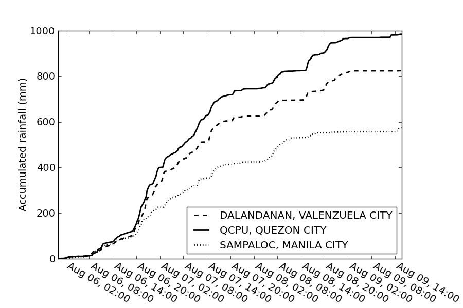
Figure 2.2: Cumulative rainfall from 6 to 9 August for three rain gauges in Metropolitan Manila. Refer to Fig. 2.1 for the position of the rain gauges. The distances between the three gauges are about 10 km.

According to Figure 2.3, three marked convective cells poured rain around Manila Bay, the largest of them extending from the centre of Manila Bay eastwards over Metropolitan Manila. Over the entire period of three days, the position of these cells remained quite persistent. This persistence––together with the high average rainfall intensities––explains the extreme local rainfall accumulations. Figure 2.3 also illustrates the mean vertical structure of rainfall between the evening of August 6 and the early morning of 7 August. The convective structures exhibit a marked decrease in rainfall intensity above an altitude of 5 to 6 km, which is typical for shallow convection. This vertical structure is also representative of the duration of the entire event.

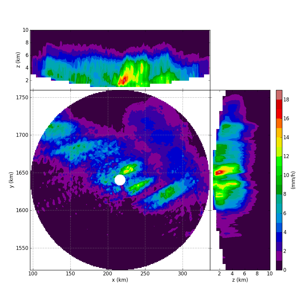
Figure 2.3: Mean rainfall intensity in the night from 6 August (20:00 UTC) until 7 August (08:00 UTC) as seen by the Subic S-band radar. The central figure shows a CAPPI at 3000 m altitude (for the rainfall estimation, we used the Pseudo-CAPPI at 2000 m. The marginal plots show the vertical distribution of intensity maxima along the x- and y-axis, respectively. In the area around Manila Bay, three marked cells appear. For these cells, the rainfall intensity exhibits a marked decrease above an altitude of 5 to 6 km, indicating rather shallow convection.

However, the unadjusted radar-based rainfall accumulation from 6 August (08:00 UTC) to 9 August (20:00 UTC) exhibits a significant underestimation if compared to the rain gauge recordings. While the radar estimates between 300 and 400 mm around Quezon City, rain gauges recorded up to 1000 mm. At the moment, the reasons for this level of underestimation remain unclear. Hardware calibration issues might as well play a role as effects of the vertical profile of reflectivity, which were not yet analysed in the course of this analysis. Beyond this general underestimation, the Subic radar shows massive beam shielding in the southern sectors, which is caused by Mount Natib, a volcano and caldera complex located in the province of Bataan. Other sectors of the Subic radar are affected by partial beam shielding due to a set of mountain peaks in the northern vicinity of the radar.

In order to correct for the substantial underestimation, rain gauge recordings were used to adjust the rainfall estimated by the radar at an altitude of 2000 m (using the mean field bias adjustment approach). This procedure reduced the crossvalidation RMSE of the event-scale rainfall accumulation by more than half. The resulting rainfall distribution is shown in Figure @ref(fig:BC_fig4). This figure gives an impressive view on the amount of rain that actually came down around Metropolitan Manila. Obviously, the actual “epicentre” of the event was situated rather over the Manila Bay than over Metropolitan Manila itself.

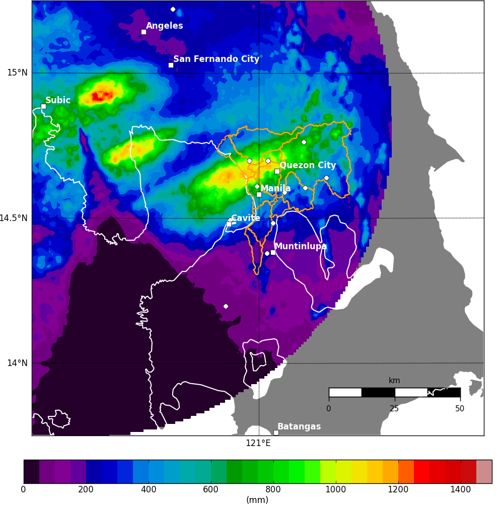
Figure 2.4: Gauge-adjusted radar-based rainfall estimation; accumulation period from 6 August (00:80 UTC) to 9 August (20:00 UTC). Basins draining to Metropolitan Manila are shown in orange, coastlines in white. Major cities are shown as white squares, while rain gages are represented as white circles. Note that the corresponding rainfall field obtained from the interpolation of rain gauge observations is available as Supplement.

Due to its size and shape, the Marikina River basin (see Figure 2.1)—as it did in September 2009—most strongly contributed to the flooding of Metropolitan Manila during the Habagat of August 2012. According to the gauge-adjusted radar rainfall estimates, the areal mean rainfall depth for the Marikina River basin amounted to 570 mm. In contrast, the areal rainfall average would add up to 440 mm (more than 20% less) if we only interpolated the rain gauge observations (by inverse distance weighting.

If we now assumed a scenario in which the rainfall field had been shifted eastward by no more than 20 km, the areal rainfall average in the Marikina River basin would have increased by almost 30%. Since the catchment had already been saturated before the onset of the main event, almost all of the additional rain would have been directly transformed to runoff. A very rough, but illustrative calculation demonstrates the potential implications: according to the extreme value statistic for the Marikina River, a 500 m\(^3\)/s increase in peak discharge at stream flow gauge Sto. Nino approximately corresponds to a 2.5-fold increase in the return period (DPWH-JICA 2003). For the Habagat of August 2012 event, the peak discharge at gauge Sto. Nino was estimated to be around 3000 m\(^3\)/s, corresponding to a return period of about 50 years. Assuming that every additional raindrop had been effective rainfall and assuming linear runoff concentration, the “20 km-shift” scenario would have resulted in a peak discharge of about 3900 m\(^3\)/s—or a return period of more than 200 years. The return period of the flood event related to Typhoon Ketsana in September 2009 was estimated to be 150 years (Tabios III 2009).

References

DPWH-JICA. 2003. “Department of Public Works and Highways, DPWH Japan International Cooperation Agency, JICA: Manual on Flood Control Planning, Project for the Enhancement of Capabilities in Flood Control.” http://www.jica.go.jp/project/philippines/ 0600933/04/pdf/Manual on FC Planning.pdf.

Tabios III, G. Q. 2009. “Marikina River Flood Hydraulic Simulation During Typhoon Ondoy of 26 September 2009.” University of the Philippines, Diliman.