4.5 Results and Discussion

The presentation and discussion of results falls into four parts.

1. In section 4.5.1, we demonstrate the effect of extending the framework of quality-weighting by path-integrated attenuation. This is done by analysing the mean and the standard deviation of differences between the two ground radars, SUB and TAG, in different scenarios of quality filtering for a case in December 2014.

2. In section 4.5.2, we construct a time series of calibration bias estimates for the TAG C-band radar by using the extended quality-averaging framework together with spaceborne reflectivity observations from TRMM and GPM overpass events. This time series complements the calibration bias estimates we had already gathered for the SUB S-band radar in Crisologo et al. (2018).

3. In section ??}, we use the calibration bias estimates for SUB and TAG in order to correct the GR reflectivity measurements, and investigate whether that correction is in fact able to reduce the absolute value of the mean difference \(\overline{\Delta Z}_{TAG-SUB}\) between the two radars. This analysis is done for events in which we have both valid SR overpasses for both radars and a sufficient number of samples between the two ground radars in the region of overlap.

4. In section 4.5.4, finally, we evaluate different techniques to interpolate the sparse calibration bias estimates in time, attempting to correct ground radar reflectivity observations also for times in which no overpass data is available. The effect of different interpolation techniques is again quantified by the mean difference \(\overline{\Delta Z}_{TAG-SUB}\) between the two ground radars.

4.5.1 The effect of extended quality filtering: the case of December 9, 2014

In this section, we demonstrate the effect of extending the quality framework by path-integrated attenuation. In Figure 4.3}, we have already seen that the SUB radar is strongly affected by beam blockage in the region of overlap. Yet, as an S-band radar, it is not significantly affected by attenuation. For the TAG radar, it is vice versa: not much affected by beam blockage, yet it will be affected by atmospheric attenuation during intense rainfall. That setting provides an ideal environment to experiment with different scenarios of quality filtering. For such an experiment, we chose a heavy rainfall event on December 9, 2014, where there are sufficient radar bins with precipitation in the region of overlap. The scan times are 06:55:14 and 06:57:58 for the SUB and TAG radars, respectively.

Figure 4.4 shows scatter plots of matched reflectivities in the region of overlap, combining matched GR bins from all elevation angles. Note that in this region of overlap, \(Q_{SUB}\) is equivalent to \(Q_{BBF}\), and \(Q_{TAG}\) is dominated by \(Q_{PIA}\). To illustrate the individual effects of the quality indices in the comparison, we simply refer to the dominating quality index instead of the associated radar (i.e. \(Q_{BBF}\) for SUB and \(Q_{PIA}\) for TAG). The points in the scatter plot are colored depending on the quality index of the corresponding matched sample: in Figure 4.4a, we can see that matches with a very low \(Q_{BBF}\) value (i.e. high beam blockage) are concentrated above the 1:1 line, since beam blockage causes the Subic radar to underestimate in comparison to the Tagaytay radar. If we consider each matched sample irrespective of data quality, the mean difference between the two radars is 1.7 dB, with a standard deviation of 8.1 dB. Taking \(Q_{BBF}\) into account changes the mean difference to -1.9 dB—which is higher in absolute terms—and decreases the standard deviation to 5.5 dB. Figure 4.4b demonstrates the effect of using only PIA for quality filtering: Points with low \(Q_{PIA}\) (i.e. high PIA) are concentrated below the 1:1 line, corresponding to an underestimation of the TAG radar as compared to the SUB radar. Considering only \(Q_{PIA}\) for quality-weighting increases the mean difference between TAG and SUB to a value of 3.5 dB, and decreases the standard deviation just slightly to a value of 7.5 dB. By combining the two quality factors, we can reduce the absolute value of \(\overline{\Delta Z}_{TAG-SUB}\) from 1.7 dBZ to -0.7 dB, and, more notably, the standard deviation from 8.1 dBZ to 4.6 dBZ (Figure 4.4c). That effect also becomes apparent in Figure 4.4d in which we show how the multiplicative combination of quality factors not only pushes the mean of the differences towards zero, but also narrows down the distribution of differences dramatically.

Remembering item (2) from section 4.3.1, it is the reduction of standard deviation that we are most interested in at this point: it demonstrates that the two GR become more consistent if we filter systematic errors that are spatially heterogeneous in the region of overlap. The low absolute value of the mean difference is, for this case study, not a result of correcting for calibration bias—which is addressed in the following sections.

On the basis of these results, we will, in the following sections, only refer to values of mean and standard deviation of (SR–GR or GR–GR) differences that are computed by means of quality-weighting, with the quality of a matched sample quantified as \(Q_{match}\).

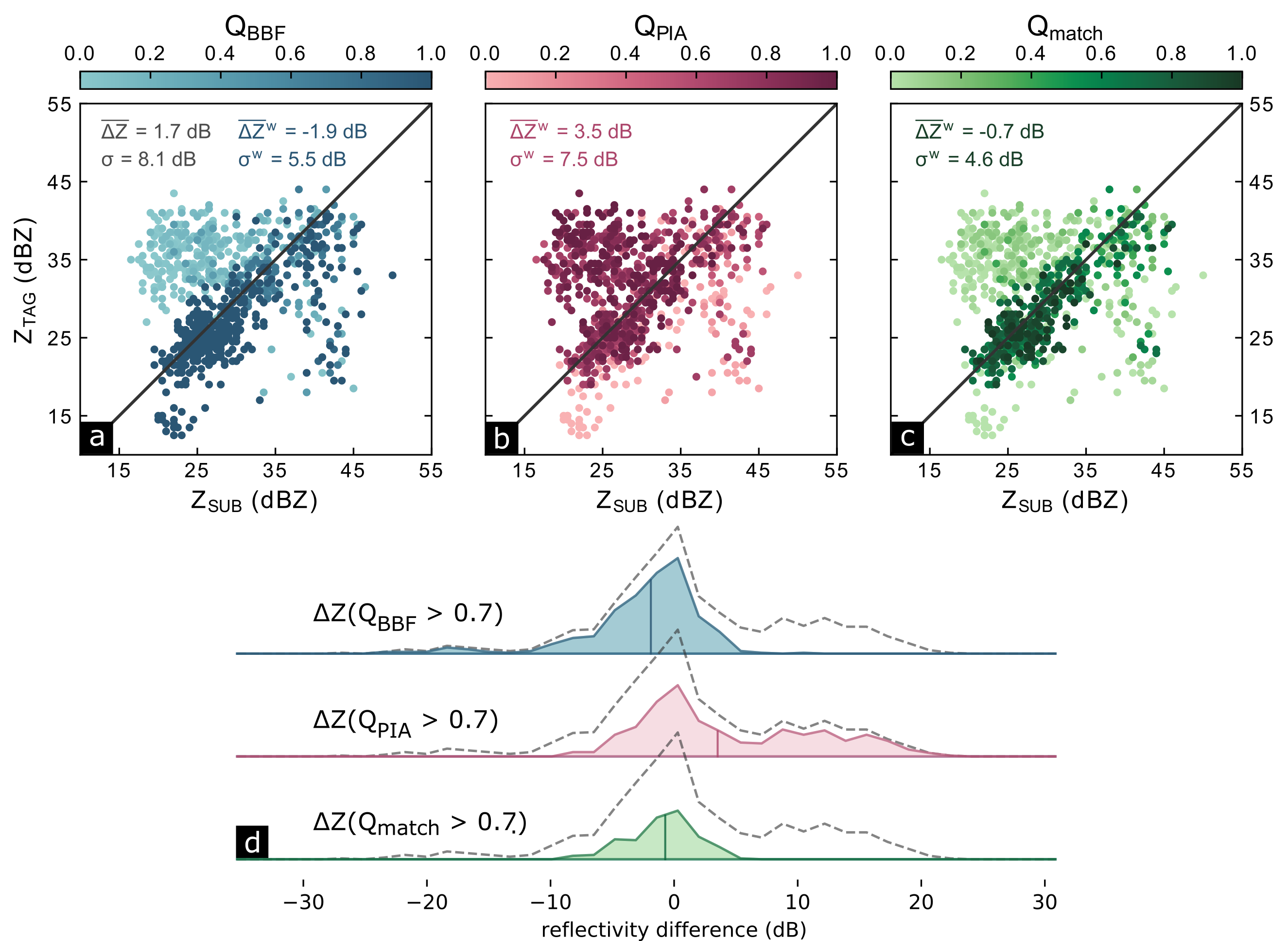
Figure 4.4: Scatter plot of reflectivity matches between Tagaytay and Subic radars. The marker color scale represents the data quality based on (a) beam blockage fraction (\(Q_{BBF}\)), (b) path-integrated attenuation (\(Q_{PIA}\)), and (c) the multiplicative combination of the two (\(Q_{match}\)), where the darker colors denote high data quality and lighter colors signify low data quality. The ridgeline plots (d) show the distribution of the reflectivity differences of the remaining points if we choose points only with high quality index (in this case, we select an arbitrary cutoff value of \(Q_{match}\) = 0.7). The mean is marked with the corresponding vertical line.

4.5.2 Estimating the GR calibration bias from SR overpass events

In Figure 8a of Crisologo et al. (2018), we had already shown the time series of quality-averaged differences between the SUB ground radar and the SR platforms TRMM and GPM, using beam blockage as a quality variable. Extending the framework for quality-weighted averaging by PIA, we have now computed the corresponding time series of quality-weighted mean differences for the TAG radar. Figure 4.5 shows the time series of calibration biases, as estimated from quality-weighted mean differences, for both SUB and TAG radars for years 2012–2014 and 2016. The first panel corresponds to Figure 8a of Crisologo et al. (2018). For SUB, there is a total of 96 SR overpass events that fit the filtering criteria referred to in Section III.2, while for TAG, we only found 45 matches. Compared to the spaceborne radars, both SUB and TAG are dramatically underestimating at the beginning of operation in 2012, where the underestimation of the TAG radar is even more pronounced. From 2014, the calibration improves for both radars.

As pointed out in Crisologo et al. (2018), there is a strong variability of the estimated calibration biases between overpasses for SUB. This behaviour can be confirmed for the TAG radar, with particularly drastic cases in 2013. Potential causes for this short-term variability have been discussed in Crisologo et al. (2018), and could include, e.g., residual errors in the volume sample intersections, short-term hardware instability, rapid changes in precipitation during the time interval between GR sweep and SR overpass, and uncertainties in the estimation of PIA, to name a few.

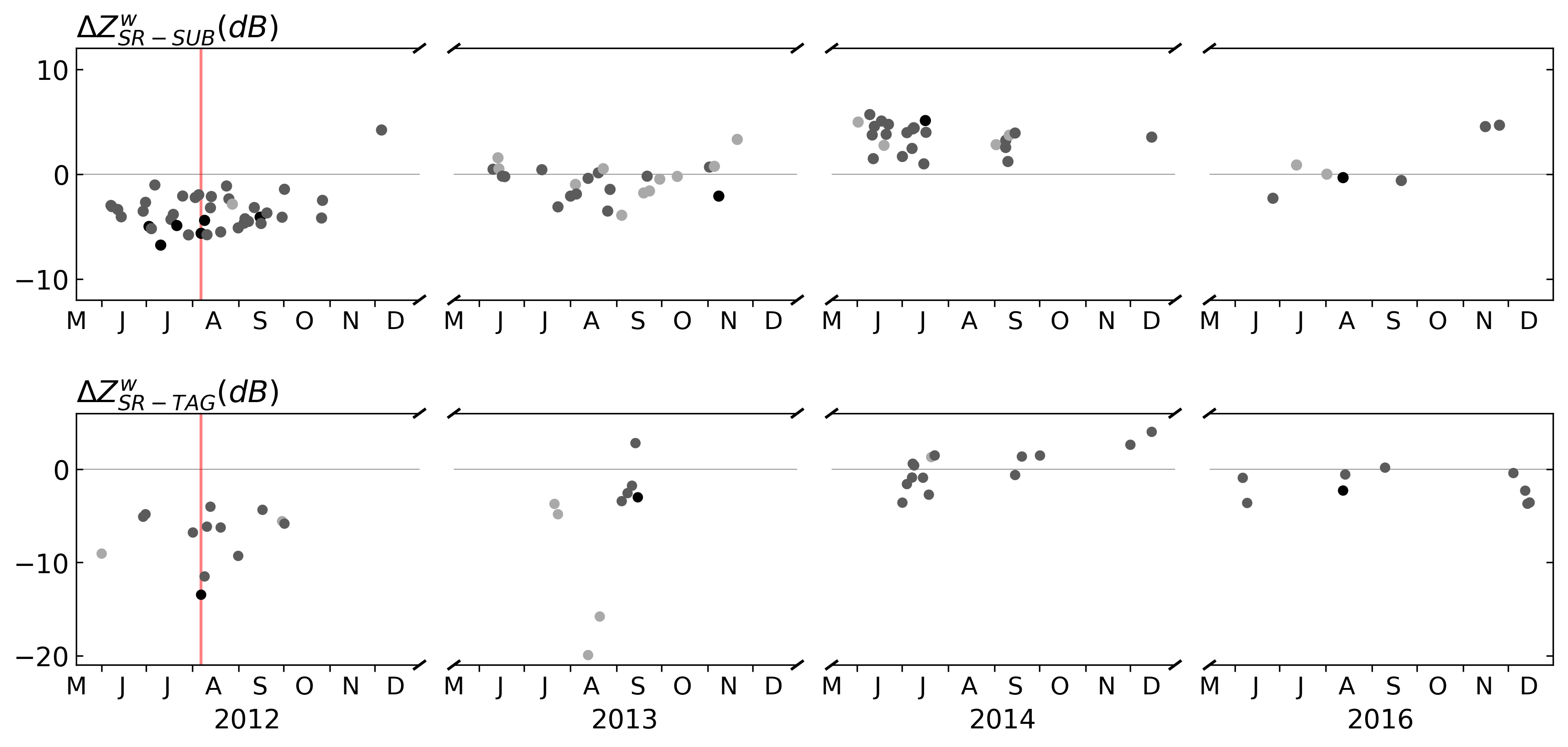
Figure 4.5: Calibration biases derived from comparison of GR with SR for SUB (a) and TAG (b) for the wet seasons (June to December) of the entire dataset. Symbols are coloured according to the number of matched samples: light grey: 10–99, medium grey: 100–999, and black: 1000+. The red line marks 06 August 2012 for the case study presented in Figure 6.

4.5.3 The effect of bias correction on the GR consistency: case studies

In this and the following section, we evaluate the effect of using the calibration bias estimates obtained from SR overpasses to actually correct the GR reflectivity measurements. We start, in this section, by analysing events in which we have both: valid SR overpass events for SUB and TAG, as well as a sufficient number of matched GR samples in the region of overlap. That way, we can directly evaluate how an “instantaneous” estimate of the GR calibration bias estimates affects the GR consistency, as explained in item (2) of section @ref(subsec:method_overview). In contrast to section 4.5.1, in which we focused on the standard deviation of differences between the two ground radars, we now focus on the mean differences in order to capture the effect of bias correction.

The first case is a particularly illustrative example: an extreme precipitation event that took place right in the region of overlap at a time in which both radars, SUB and TAG, apparently were affected by massive miscalibration, according to Figure 4.6 the so-called Habagat of 2012, an enhanced monsoon event that happened in August 2012 (M. Heistermann et al. 2013).

Figure 4.6a and b illustrate the estimation of the calibration bias for the SUB and TAG radars from TRMM overpass data. The calibration bias estimates of -5.6 dB (for SUB) and -13.5 dB (for TAG) obtained from those scatter plots correspond to the dots intersecting the red line in the time series shown in Figure 4.5. Figure 4.6c shows the matching reflectivity samples of the two ground radars, SUB and TAG, in the region of overlap which have not yet been corrected for calibration bias. The quality-weighted mean difference of reflectivies amounts to -12.2 dB. Accordingly, Figure 4.6d shows the matches in the region of overlap, with both SUB and TAG reflectivities corrected for calibration bias, based on the values obtained from Figure 4.6a and b, respectively. The corresponding value of the mean difference amounts to -4.6 dB. These effects are further illustrated by Figure 4.6e which shows the distributions of SR–GR and GR–GR differences before and after bias correction.

The case clearly demonstrates how massive levels of miscalibration (-5.6 and -13.5 dB) can be reduced if an adequate SR overpass is available. That is proved by the massive reduction of the absolute value of mean difference between the two ground radars, or, inversely, the massive gain in GR consistency. Yet, the bias could not be entirely eliminated, which suggests that other systematic sources of error have not been successfully addressed for this case.

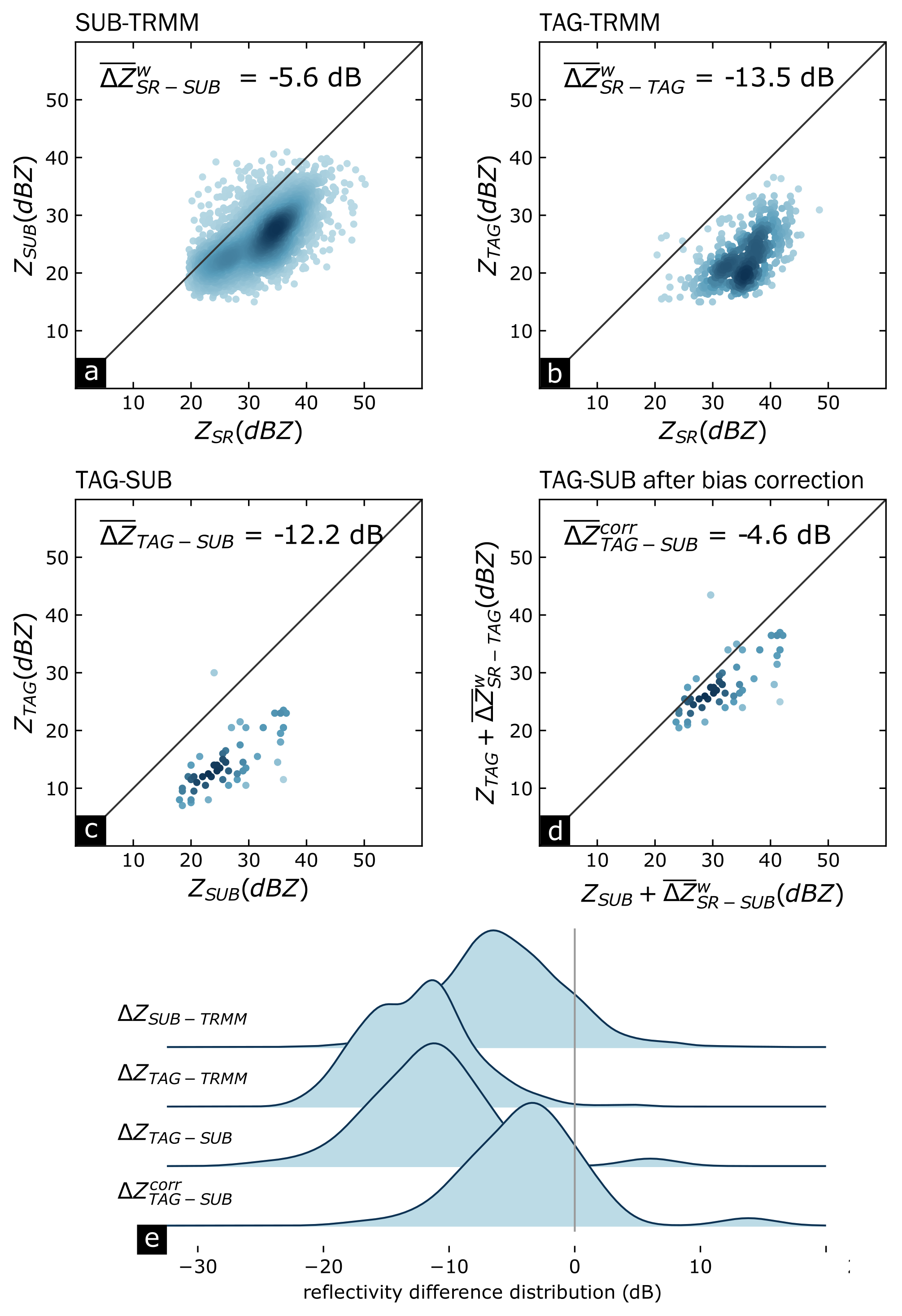
Figure 4.6: 3-way case study for 2012-08-06 17:15:47. (a) and (b): Scatter plots of SR–GR comparisons between TRMM and SUB and TAG radars for points where \(Q_{match}\)>0.7, where the darkness of the color represents the point density. The corresponding weighted biases are calculated for each radar. (c) and (d): GR–GR inter-radar consistencies before and after bias correction. (e) Distribution of the differences of the reflectivity pairs for each comparison scenario.

Table 4.2 summarizes our analysis of five additional events in which valid SR overpasses for both SUB and TAG coincided with a significant rainfall in the region of overlap between the two ground radars, most of which took place in 2012 (and one in 2016). Columns \(\overline{\Delta Z}^w_{SR-SUB}\) and \(\overline{\Delta Z}^w_{SR-TAG}\) show varying levels of calibration bias for SUB and TAG, quantified by the quality-weighted mean difference to the SR observations, together with varying levels of mismatch between the two ground radars, as shown by column \(\overline{\Delta Z}^{no corr}_{TAG-SUB}\). Using the calibration bias estimates for correcting the GR observations, we consistently reduce the quality-weighted mean difference between both ground radars, as expressed by column \(\overline{\Delta Z}^{w,corr}_{TAG-SUB}\).

Table 4.2: Calibration biases and inter-radar consistencies for different bias calculation scenarios

	Npts	DZw SR-SUB	DZw SR-TAG	DZnocorr TAG-SUB	DZw TAG ,corr -SUB
2012-06-11 21:37:41	528	-3.4	-6.3	-3.5	-0.2
2012-06-28 22:14:46	48	-3.5	-5.1	-1.3	-0.2
2012-07-02 20:09:47	1248	-5	-11.4	-7	-2.1
2012-07-02 20:09:47	1248	-5	-11.4	-7	-2.1
2012-08-31 13:44:31	34	-5.1	-9.3	-1.9	1.1
2016-08-12 11:40:28	1277	-0.3	-2.3	-5.7	-4.3

Altogether, the correction of GR reflectivities with calibration bias estimates of SR overpasses dramatically improves the consistency between the two ground radars which have shown largely incoherent observations before the correction. In all cases (including the Habagat of 2012), we were able to reduce the mean difference between the ground radars.

The question is now: Can we use these sparse calibration bias estimates also for points in time in which no adequate SR overpass data are available? Or, in other words, can we interpolate calibration bias estimates in time?

4.5.4 Can we interpolate calibration bias estimates in time?

The spaceborne radar platform (SR) rarely overpasses both GR radar domains in a way that significant rainfall sufficiently extends over both GR domains including the GR region of overlap. Hence, our previous demonstration of the effective correction of GR calibration bias yielded only few examples. From a more practical point of view, however, we are more interested in how we can use SR overpass data for those situations in which adequate SR coverage is unavailable—which is, obviously, rather the rule than the exception. An intuitive approach is to interpolate the calibration bias estimates from valid SR overpasses in time, and use the interpolated values to correct GR observations for any point in time. We can do such an interpolation independently for each ground radar, based on the set of valid SR overpasses available for each. In order to examine the effectiveness of such an interpolation, we again use the absolute value of the mean difference between the two ground radars as a measure of their (in-)consistency. Based on the reduction of that absolute value, as compared to uncorrected GR reflectivities, we benchmark the performance of three interpolation approaches:

1. Linear interpolation in time;
2. Moving average: we compute the calibration bias at any point in time based on calibration bias estimates in a 30-day window around that point, together with a triangular weighting function;
3. Seasonal average: For any point in time in the analyzed wet season of a year, we compute the calibration bias as the average of all calibration bias estimates available in that year.

This benchmark analysis is not considered to be comprehensive, but rather exemplary in terms of examined interpolation techniques. The three techniques illustrate different assumptions on the temporal representativeness of calibration bias estimates, as obtained from SR overpasses: a seasonal average reflects a rather low level of confidence in the temporal representativeness. The underlying assumption would be that we consider any short-term variability as “noise” which should be averaged out. The linear interpolation puts more confidence into each individual bias estimate, and assumes that we can actually interpolate between any two points in time. Obviously, a 30-day moving average is somewhere in between the two.

Table 4.3: Mean absolute \(\Delta Z_{TAG-SUB}\) for different correction scenarios and years

	No correction	Seasonal mean	Linear interpolation	Moving average
All years	4.9	4.0	3.0	2.7
2012	4.4	3.4	2.6	2.3
2013	8.6	7.1	4.5	4.1
2014	4.4	3.8	3.2	2.9
2016	1.8	1.8	1.7	1.7

Table 4.3 provides an annual summary of the absolute mean differences in reflectivity between the two ground radars, without bias correction and with correction of bias obtained from different interpolation techniques. Firstly, the mean absolute difference between the radars is always lower after correction, irrespective of the year or the interpolation method. Hence, it is generally better to use calibration bias estimates to correct GR reflectivities even for those times in which no valid SR overpasses are available. The 30-day moving average appears to outperform the other two interpolation methods—on average, and for each year from 2012 to 2014. In 2016, neither interpolation method substantially reduces the mean absolute difference obtained for the uncorrected GR data.

The performance of the moving average suggests that it is possible for the calibration of radars to drift slowly in time, with variability stemming from sources which are difficult to disentangle. However, for periods of time when the radar is relatively well-calibrated and stable, the bias correction only offers a slight, if any, improvement in the consistency between two radars.

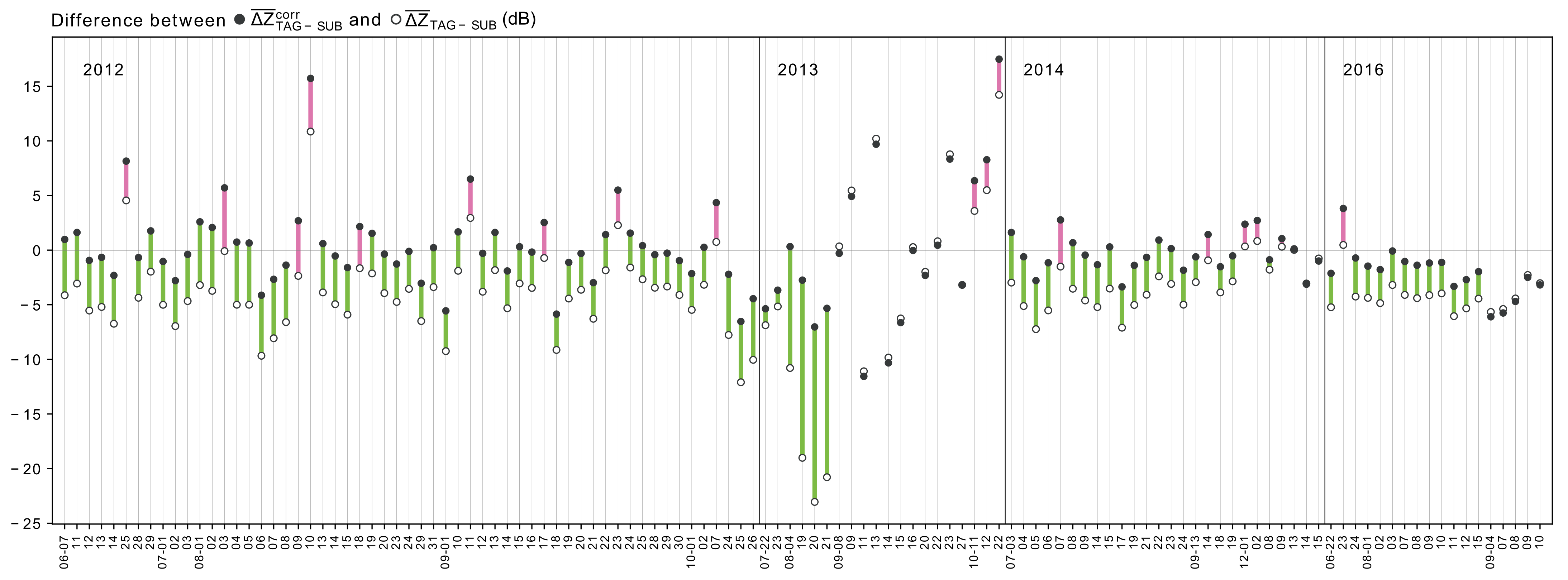
Figure 4.7: The differences between the inter-radar consistency before and after correcting for the ground radar calibration biases following a rolling window averaging for samples with significant number of matches. The hollow (filled) circles represent the daily mean before (after) correction. The line color represents an improvement (green) or a decline (pink) in the consistency between the two ground radars.

In order to better understand the variability “behind” the annual averages in Table 4.3, Figure 4.7 shows the effects of bias correction on a daily basis, exemplified for the moving average interpolation. The hollow circles represent the daily mean differences between the two ground radars before (\(\overline{\Delta Z}_{TAG-SUB}\)) correction, while the filled circles show the daily mean differences after (\(\overline{\Delta Z}^{w,corr}_{TAG-SUB}\)) correction. The length of the bar shows the magnitude of the change, while the color of the bar signifies a reduction of the absolute value of the mean difference (green, for improvement) or an increase in in the absolute value (pink, for a degradation of consistency between the two ground radars). In 83 out of 121 days, bias correction improves the consistency between the two ground radars by more than 1 dB. Inversely, though, this implies that in 17 out of 121 days, the use of interpolated bias estimates causes a degradation of consistency between the ground radars, expressed as an increase of more than 1 dB in the absolute mean differences. Furthermore, we can identify several days for which the bias correction decreases the absolute mean differences, but not to a level that could be considered as acceptable for quantitative precipitation estimation.

In 2011, Schwaller and Morris had presented a technique to match reflectivity observations from spaceborne radars (SR) and ground radars (GR). Crisologo et al. (2018) extended that technique by introducing the concept of quality-weighted averaging of reflectivity in order to retrieve the GR calibration bias from matching SR overpass data. They exemplified the concept of quality weighting by using beam blockage as a quality variable, and demonstrated the effectiveness of the approach for the Subic S-band radar in the Philippines.

The present study has extended the concept of quality-weighted averaging by accounting for path-integrated attenuation (PIA) as a quality variable, in addition to beam blockage. Accounting for PIA becomes vital for ground radars that operate at C- or X-band. In addition to the Subic S-band radar, this study has included the Tagaytay C-band radar which substantially overlaps with the Subic radar.

In the first part of this study, we have demonstrated that only accounting for both, beam blockage and path-integrated attenuation, allows for a consistent comparison of observations from the two ground radars, Subic and Tagaytay: after transforming the quality variables “beam blockage fraction” and “path-integrated attenuation” into quality indices \(Q_{BBF}\) and \(Q_{PIA}\), with values between zero and one, we computed the quality-weighted standard deviation of matching reflectivities in the region of overlap between the two ground radars for an event on December 9, 2014. Using a quality index based on the multiplicative combination of \(Q_{BBF}\) and \(Q_{PIA}\), we were able to dramatically reduce the quality-weighted standard deviation from 8.1 dBZ to 4.6 dBZ, while using \(Q_{BBF}\) and \(Q_{PIA}\) alone would have only reduced the standard deviation to 5.5 or 7.5 dBZ, respectively. Based on that result, we have used, with confidence, the combined quality index throughout the rest of the study.

The next step involved the retrieval of the GR calibration bias from SR overpass data for the Tagaytay C-band radar (for the Subic S-band radar, that had already been done by Crisologo et al. (2018)). For each matched volume in the SR–GR intersection, the combined quality index was computed for the Tagaytay radar, and used as weights in calculating the calibration bias as a quality-weighted average of the differences between SR and GR reflectivities. We applied this approach throughout a 4-year period to come up with a time series of the historical calibration bias estimates of the TAG radar, and found the calibration of the TAG radar to be exceptionally poor and volatile in the years 2012 and 2013, with substantial improvements in 2014 and 2016.

In order to demonstrate the effectiveness of estimating and applying the GR calibration bias obtained from SR overpass data, we have compared, in the region of overlap, the corrected and uncorrected reflectivities of the Subic and Tagaytay radars, for six significant rainfall events in which all three instruments—TAG, SUB and the SR—had recorded a sufficient number of observations. We have shown that the independent bias correction is able to massively increase the consistency of the two ground radar observations, as expressed by a reduction of the absolute mean difference between the GR observations in the region of overlap, for each of the six events—in one case even by almost 7.7 dB. The main lesson from these cases is, that we can legitimately interpret the quality-weighted mean difference between SR and GR reflectivities as the instantaneous GR calibration bias, even if the magnitude of that bias varies substantially within short periods of time.

Yet, the question remains how to correct for calibration bias in the absence of useful SR overpasses. That question is particularly relevant for the reanalysis of archived measurements from single-pol weather radars. In this study, we have evaluated three different approaches to interpolate calibration bias estimates from SR overpass data in time: linear interpolation, a 30-day moving average, and a seasonal average. Each of these approaches illustrates different assumptions on the temporal representativeness of the calibration bias estimates. On average, any of these approaches produced calibration bias estimates that were able to reduce the mean absolute difference between the GR observations, which increases our confidence in the corrected GR observations. Of all interpolation approaches, the moving 30-day window outperformed the other two approaches. However, we also found that behind the average improvement of GR–GR consistency, there were also a number of cases in which the consistency between the ground radars was degraded, or in which high inconsistencies could not be significantly improved. Altogether, it still appears difficult to interpolate such a volatile behaviour, even if we consider the actual calibration bias estimates from the SR overpasses as quite reliable.

In that context, maintenance protocols of the affected ground radars would be very helpful in interpreting and interpolating time series of calibration bias estimates. Such records were unavailable for the present study, which made it hard to understand the observed variability of calibration bias estimates. Yet, this information will mostly be internally available at those institutions operating the weather radars. With the software code and sample data of our study being openly available (), such institutions are now enabled to carry out analyses as the present study themselves, while being able to benefit from cross-referencing the results with internal maintenance protocols.

The correction of GR calibration appeared particularly effective in periods with massive levels of miscalibration. For such cases, interpolated bias estimates allowed for an effective improvement of raw GR reflectivities. Yet, we need to continue disentangling different sources of uncertainty for both SR and GR observations in order to separate actual variations in instrument calibration and stability from measurement errors that accumulate along the propagation path, and to better understand the requirements to robustly estimating these properties from limited samples. Progress on these ends should also improve the potential for interpolating calibration bias estimates in time, in order to tap the potential of historical radar archives for radar climatology, and to increase the homogeneity of composite products from heterogeneous weather radar networks.

References

Crisologo, Irene, Robert A. Warren, Kai Mühlbauer, and Maik Heistermann. 2018. “Enhancing the Consistency of Spaceborne and Ground-Based Radar Comparisons by Using Beam Blockage Fraction as a Quality Filter.” Atmospheric Measurement Techniques 11 (9): 5223–36. https://doi.org/https://doi.org/10.5194/amt-11-5223-2018.

Heistermann, M., I. Crisologo, C. C. Abon, B. A. Racoma, S. Jacobi, N. T. Servando, C. P. C. David, and A. Bronstert. 2013. “Brief Communication "Using the New Philippine Radar Network to Reconstruct the Habagat of August 2012 Monsoon Event Around Metropolitan Manila".” Nat. Hazards Earth Syst. Sci. 13 (3): 653–57. https://doi.org/10.5194/nhess-13-653-2013.